Performance charts – MagicOpt vs hyperopt
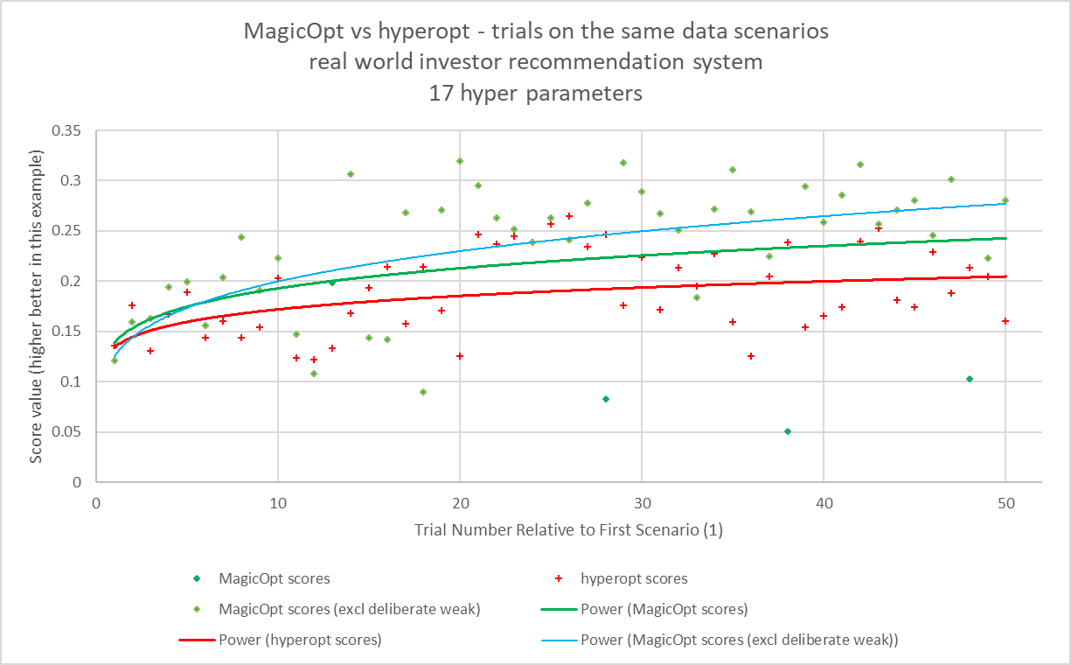
The chart above shows the first 50 trials of the same real world scenario with MagicOpt and hyperopt. The green diamonds represent MagicOpt scores at each trial. The red plus marks indicate hyperopt scores for the corresponding trial.
The blue line shows the resulting score trend when MagicOpt is evaluated only for the roughly 80% of trials where it is trying to predict a generally high score.
The green line shows the resulting score trend when all MagicOpt trials are considered.
The red line shows the resulting score trend when all hyperopt trials are considered.
As you can see, MagicOpt quickly pulls away and even expands its lead. This results in faster time to a high quality score and confidence that the search space was explored and learned effectively.
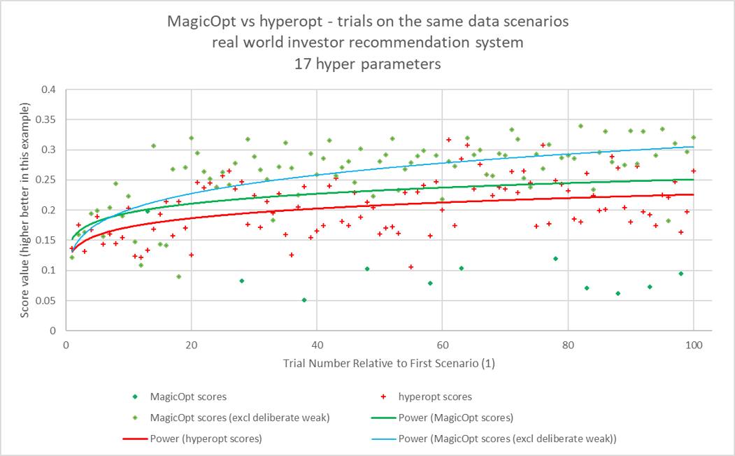
The charts below show this trend is sustained beyond the first 50 trials.
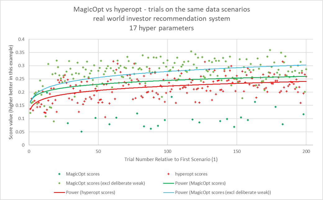
And one more chart shows the gap continues even to 200 trials. For this optimization challenge 200 trials are usually not used, as it takes several days to compute and strong values from MagicOpt are apparent earlier.
Let’s Jump In.
MagicOpt represents a leap beyond typical hyperparameter optimization. Using “experience” in combination with grid or random search doesn’t perform well enough. It’s certain you will miss something from time to time. For expensive or time consuming tests, you’ll spend more time and resources than necessary.
hyperopt represents a popular type of open source tool. The python based Bayesian optimizer is a significant improvement over simple grid search methods.
However, this type of approach learns its space more slowly than necessary while appearing to incrementally approach the first apparent optimum it senses.
We’ll compare MagicOpt with hyperopt for a real world recommender system with 17 hyper parameters. Although MagicOpt is a more powerful hyper optimizer, we still give kudos to hyperopt and its authors for their contribution to the state of the art.
MagicOpt has a dual goal with each trial. Clearly, one goal is to maximize the score quality (either minimizing or maximizing a value). The other goal is to learn as much as possible about the impact of the hyper parameter space, including its interactions and sensitivities, in each trial. In practice, you see a wider variation and more effective learning of the system being optimized.
The scatter charts show sequential trials and their resultant scores for both MagicOpt and hyperopt. These were both run on the same problem and same data scenarios. Each successive trial uses a distinct subset of available data for training and validation. Both engines saw the exact same data at each trial, though it varies from trial to trial.
The red plus marks show trial outcomes for hyperopt. You can see they are less varied, with fewer very low values and fewer high values. The red line is a power curve fit to these points.
The green diamonds show trial outcomes for MagicOpt. You can see much more variance, with some extremely low scores, more in the midrange, and a cluster at high values, typically above the values reached by hyperopt. The green line is a power curve fit to these points.
Since MagicOpt trials are not usually seeking the highest outcome, and some are specifically seeking weaker outcomes, its data points are separated into a group of all trials and a subset group that excludes deliberately weak exploration trials. The blue line shows the power curve of the MagicOpt trials that were predicted to expose high scores. This represents roughly 80% of all MagicOpt trials, though the greediness does self-adjust.