MagicOpt Performance
Extreme Optimization with MagicOpt
February 2020
– The Birth of MagicOpt
Our team faced significant optimization problems. For example, we had a powerful model with twenty hyperparameters and an evaluation cycle that took hours per trial. Tuning was challenging, even though we were running tightly optimized code on a large pool of processors to minimize training cycle time. The tools limited us.
We used in-house tools and open-source Bayesian optimizers. Something was being left on the table. We looked at commercial offerings, but they were too consultative and too expensive.
A project to dramatically, automatically, and cost-effectively improve the hyperparameter optimization process was born. We call it MagicOpt.
It is not Magic, just Math, but the results seem like magic.
Repeated Trials Tell the Story
There are some problems in parameter tuning where new candidate values can be tested in milliseconds or seconds. For those problems, where thousands of trials are practical, standard methods like random search, open-source Bayesian solutions, or even grid search in some cases, may work fine.
This is not why we are here. We are trying to select “optimal” and “stable” parameters where minor differences are costly, where validation time or cost is high, where confidence in the chosen selection is crucial.
MagicOpt is for substantive, real-world optimization problems.
Establishing a Baseline
To demonstrate that MagicOpt outperforms other methods, we perform bake-offs against alternatives with real-world problems and a library of optimization-function challenges that are representative of real-world situations.
We’ve tested MagicOpt on thousands of optimization scenarios. We’ve compared it extensively to open source solutions and random grid search.
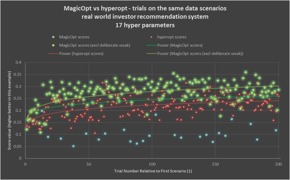
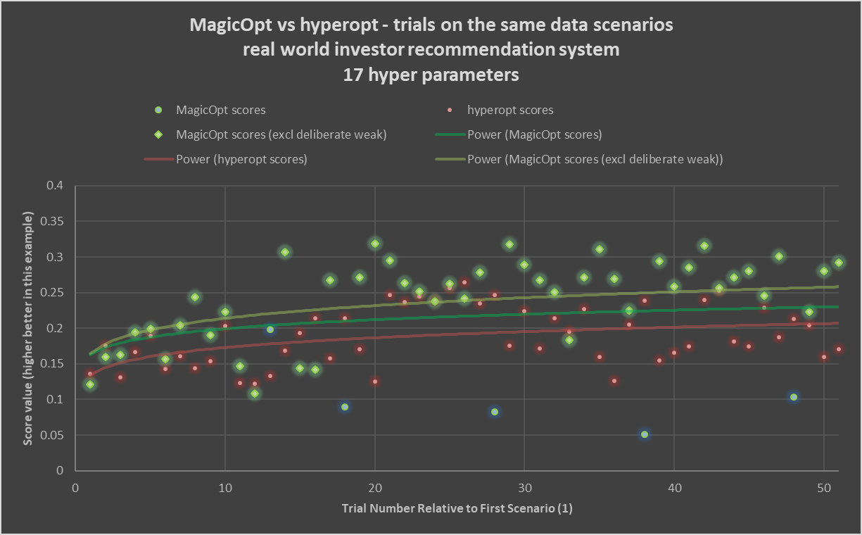
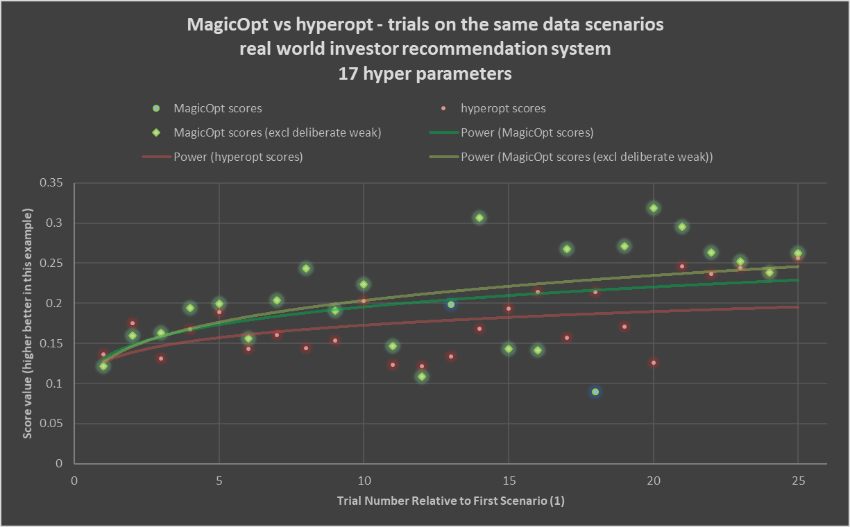
The chart above shows typical results from a real-world project. In this case, 200 trials (rotate to zoom earlier) are run with MagicOpt and Hyperopt, a common open-source Bayesian optimizer.
The glowing green diamonds show results of MagicOpt trials where it is trying for a generally strong score. The soft teal circles are results of MagicOpt trials where it is exploring and deliberately trying to find weaker or midrange outcomes. The red circles are successive trials by hyperopt. The light-green, darker-green, and red lines show power-curve fits for MagicOpt gain seeking, MagicOpt overall (including the deliberately weaker attempts) and Hyperopt, respectively. You can clearly see a large gap forms between the trial expectations of MagicOpt and Hyperopt.
More Situations, More Trials
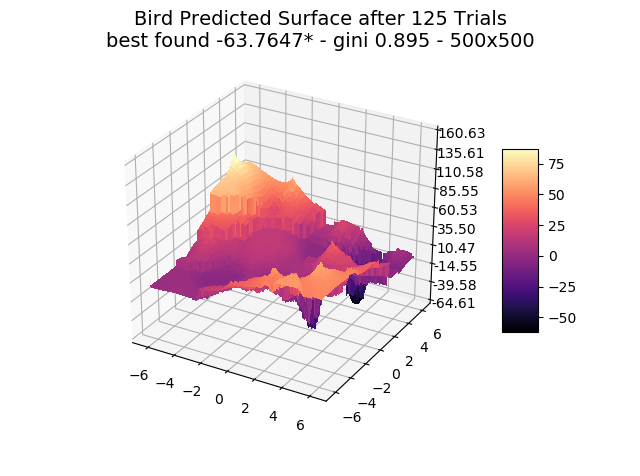
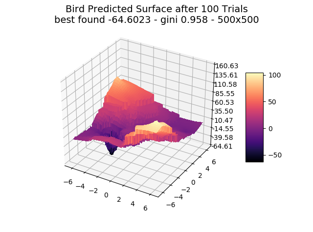
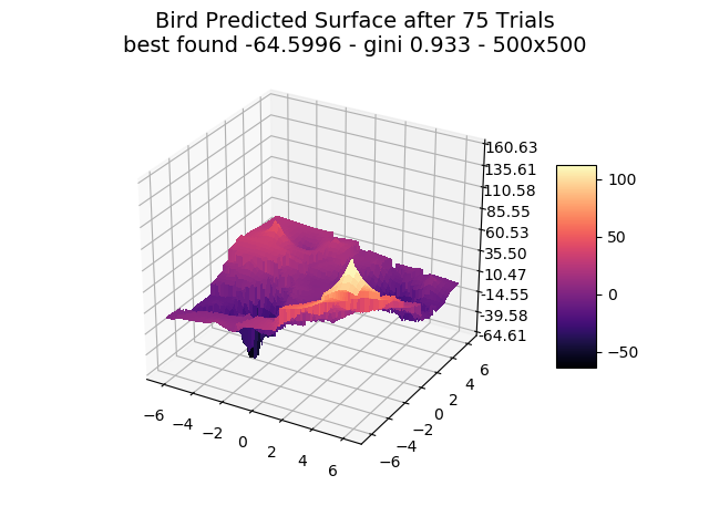
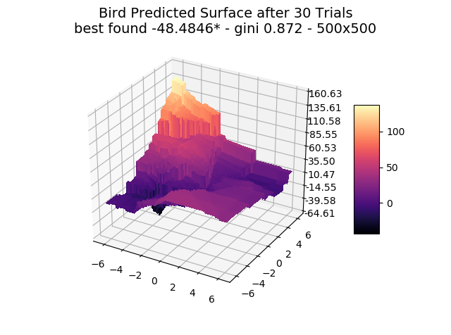
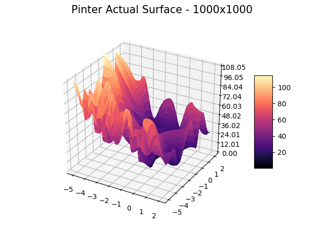
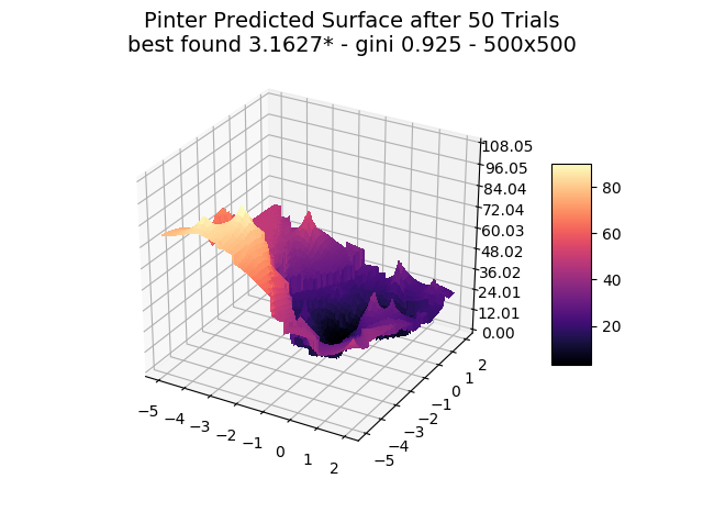
The Optimization Landscape
MagicOpt has been tested with thousands of optimization “surfaces” with one to hundreds of dimensions.
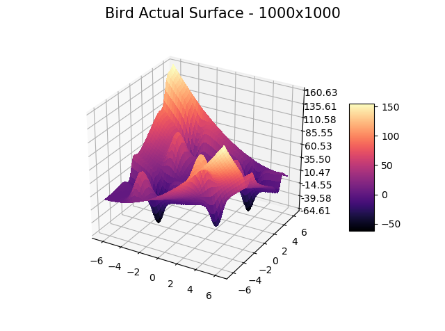
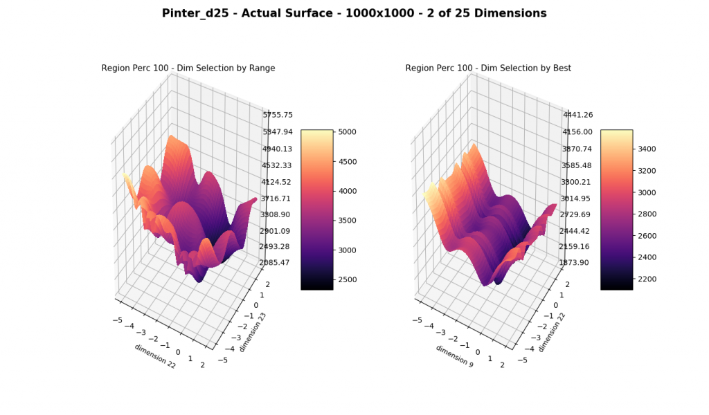
We show a few interesting cases below, sticking mainly to two dimensions for simplicity.
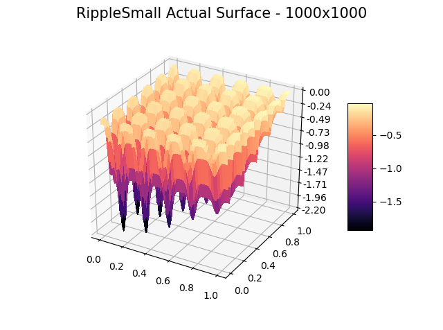
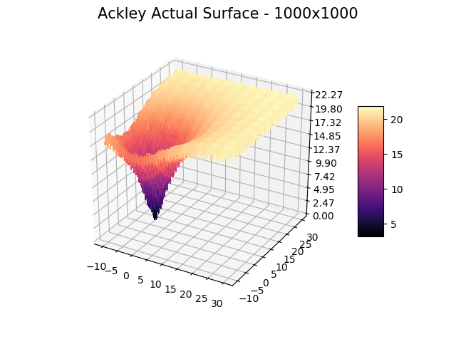
We include ‘actual’ charts of the surfaces based on a million samples in a 1000×1000 grid search. This is for illustration only, as real-world models are too costly to execute or have too many dimensions for a grid search.
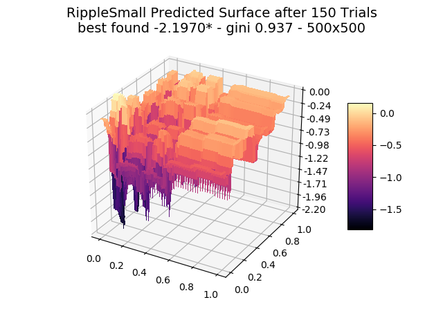
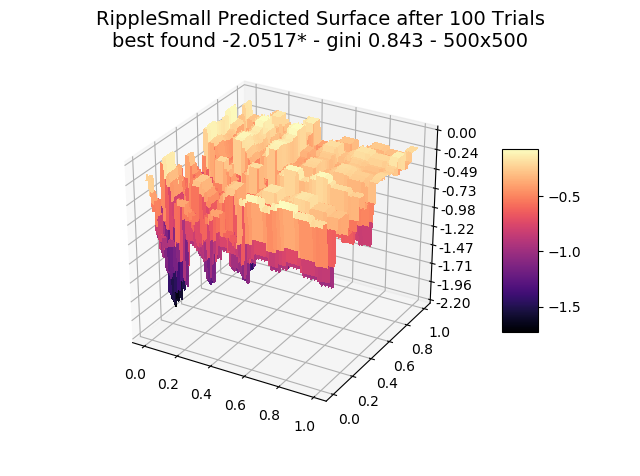
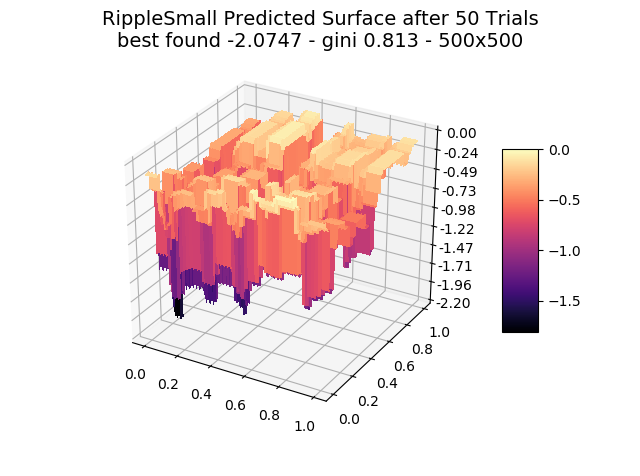
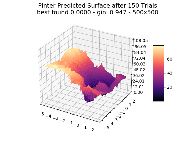
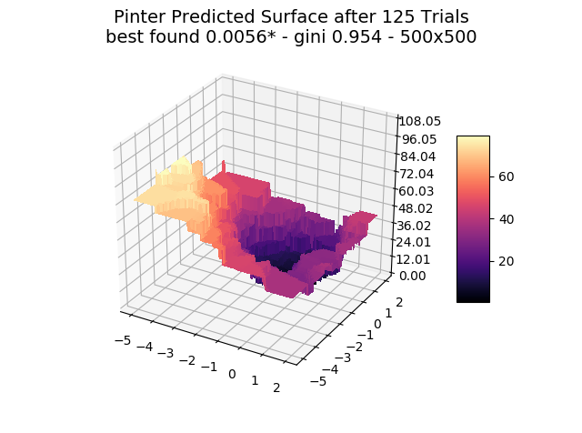
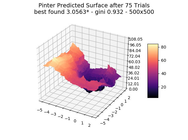
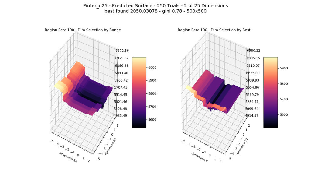
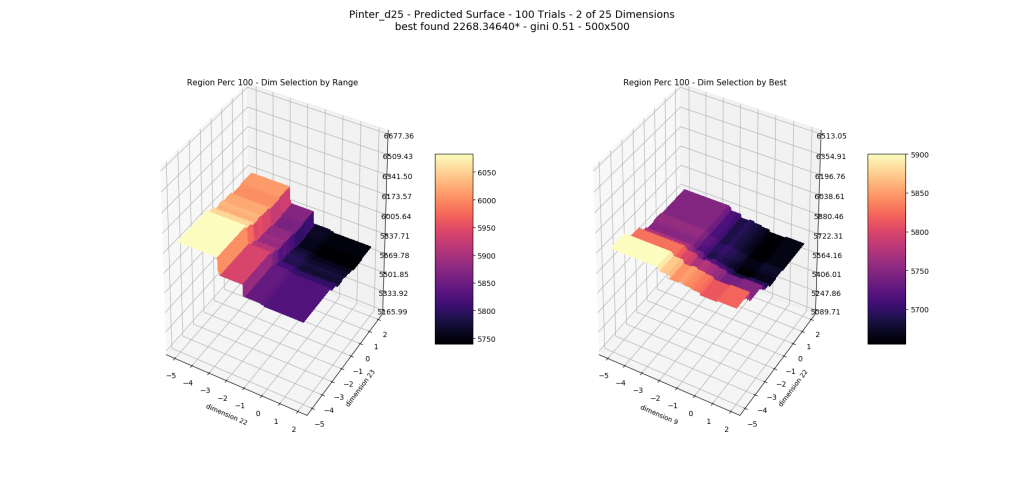
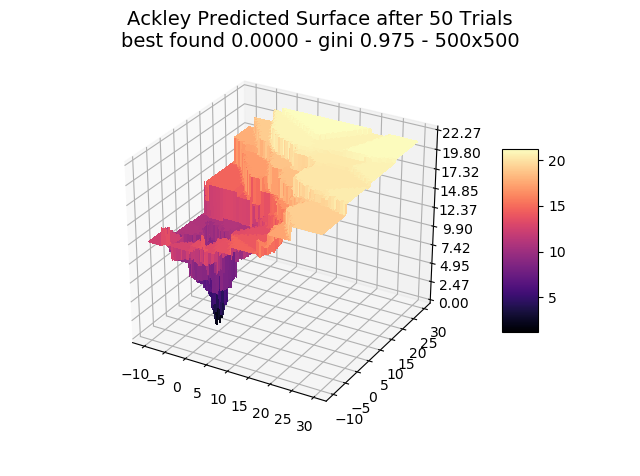
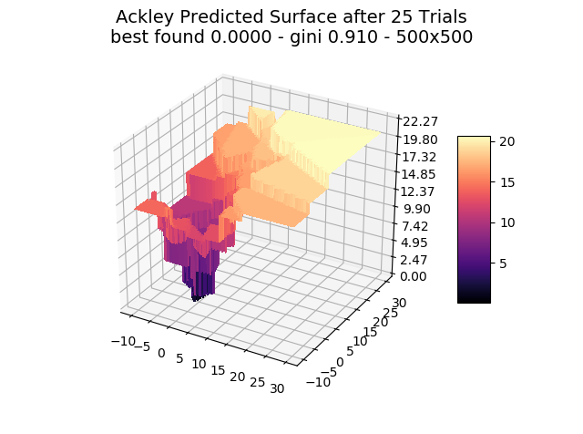
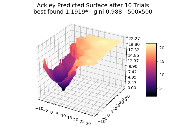
The optimizer starts with zero information on the actual surface. It learns through the feedback from its trials.
Browse through the images to see how MagicOpt views these surfaces after varying numbers of trials. You will see how quickly MagicOpt learns complex problems! The image doesn’t need to converge to find the optima, but it is a good indication of learning progression. Most examples are from 2 parameter surfaces, where it is easiest to visualize. Some also include examples at 25 and 50 dimensions (using a reduced dimension view).
The complexity of these surfaces, and the literally unlimited number of forms in the real world, illustrate the challenge of optimization. In optimization challenges with multiple objectives, each objective can see a different type of surface. The images demonstrate that MagicOpt learns extremely efficiently and forms a representative view of the solution space.
A quick note that we hope you assumed: MagicOpt isn’t tuned or modified for any specific test case, test suite, or surface characteristics. It is a general optimization framework that starts each problem with a blank slate. The only minor exception is our long-term optimization option, which can learn from your past projects to accelerate future projects that you classify similarly.
MagicOpt Finds Better Solutions, Faster
On our real-world problem set and hundreds of complex surfaces, we bench-marked MagicOpt against two real-world competitors. We chose ‘Hyperopt,’ an open-source Bayesian optimizer, and random search with a 2X trial count advantage.
All three have the same exact scenarios and start with only the hyperparameter schema.
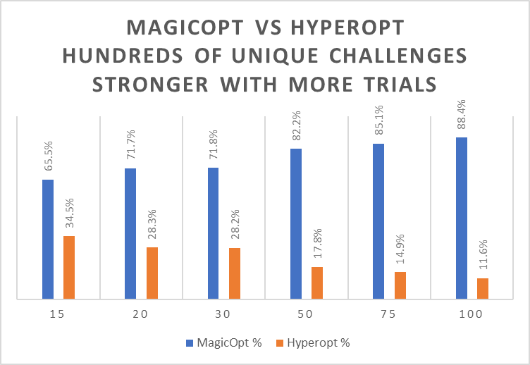
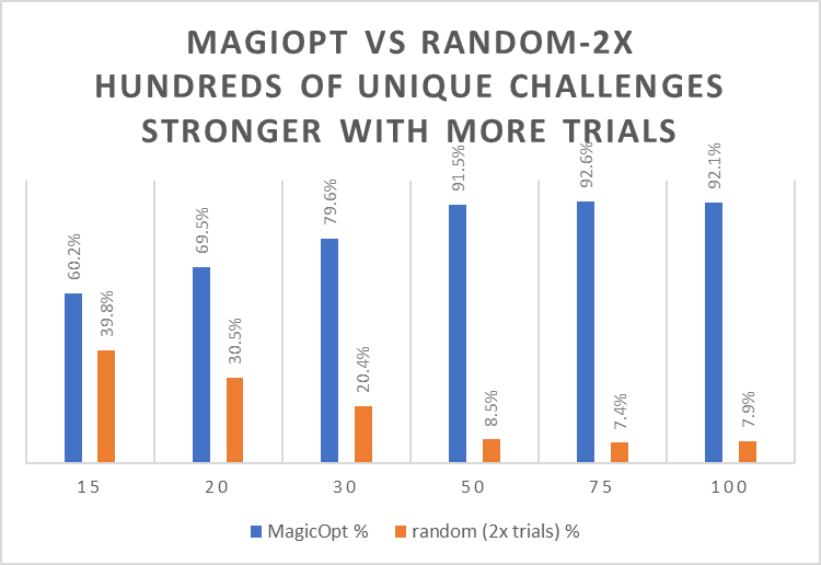
MagicOpt Starts out Better, and then pulls away!
In the charts above, you can see how MagicOpt performs against the alternatives when various numbers of trials are allowed.
Since random search is used when trial iterations are cheap, we give it twice as many trials as MagicOpt or Hyperopt in these comparisons. That raises the bar with a small edge given to random search.
The main takeaway is that MagicOpt beats Hyperopt or random search (at 2x trials) 75-90% of the time. This shows the advantage is robust across a wide range of optimization scenarios. The more trials, the more MagicOpt pulls away!
At trial counts of 200 and above (this is not shown on the charts above), MagicOpt beats random 80-90% of the time when random gets 10X the trials. Only 200 trials with MagicOpt will outperform 2000 random trials 80-90% of the time!